You have reached the updated cMonkey site with a new R package, installation and running instructions, and additional information.

If you are looking for the original cMonkey site, you can find it here. The original cMonkey algorithm was published with the manuscript “Integrated biclustering of heterogeneous genome-wide datasets for the inference of global regulatory networks”, by David J Reiss, Nitin S Baliga and Richard Bonneau.

*NEW* cMonkey package and source code are now on Github.

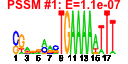
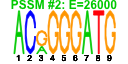
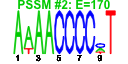
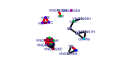
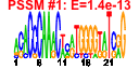
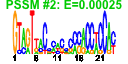
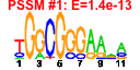
organism	n.genes	n.arrays	profile	network	motif1	motif2	motif.posns
S. cerevisiae	12	445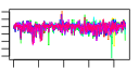
E. coli	24	329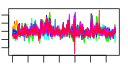
H. pylori	12	36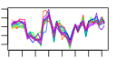
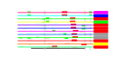H. salinarum	21	175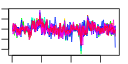
A. thaliana	19	66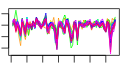

SUMMARY

The latest version of cMonkey is still under active development and has now been applied successfully to many systems, including plants (Arabidopsis thaliana) and mammals (Homo sapiens).

The cMonkey package will enable a user to run the integraged biclustering algorithm on their own microarray data, for their own organism of interest. During initialization, it will automatically download and integrate additional data for that organism, including:

genome sequence data (from RSAT) in the form of:
- genome sequence and promoter sequences
- gene annotations and coordinates
operon data and predictions (from MicrobesOnline)
functional associations between genes from one or more of:
gene functional annotations from NCBI COG
coming soon: GO annotations and KEGG annotations and pathways will be automatically included as well.
Additional user-defined data sets from local files, such as protein-protein and protein-DNA interactions, annotations, etc. may be easily integrated as well.

IMPORTANT NOTE: cMonkey currently does not completely support H. sapiens. We are working on a version for that specific task. In the meantime, see below for instructions on using cMonkey to run only on your Hsa expression data (i.e. without motifs or networks).

INSTALLATION

To run cMonkey on your own expression data, you will need to use a UNIX-y operating system (e.g., Mac OS-X or Linux). cMonkey is not currently supported on Windows. For Windows users, Cygwin, VirtualBox, or Amazon AWS are inexpensive options to obtain access to a UNIX system.

You will only need to do the following steps once:

Install the latest version of R (I am currently using version 2.11.0). It should work for versions 2.9.x and up.
Install the following R packages and their dependencies (all are helpful, but none are absolutely required): RCurl, doMC, igraph0, RSVGTipsDevice, and hwriter by typing in R:
```
install.packages(c('RCurl', 'doMC', 'igraph0', 'RSVGTipsDevice', 'hwriter'))
```
- The latter three packages are used only for plotting and graphical output.
- * NOTE the doMC package for multi-processor parallelization will not work when using the R GUI in Mac OS X. If you want cMonkey to utilize all processors/cores on your machine, run R from a terminal instead. Also NOTE that the doMC package only works on UNIX OSes (e.g. Linux or Mac OS X).
Install the cMonkey package from Github using devtools. In R, type:
```
install.packages('devtools', dep=T)
require(devtools)
install_github('cmonkey', 'djreiss', subdir='cMonkey')
```
* NOTE while the package will install correctly, it generates warnings during installation. Also NOTE that the inline documentation is currently empty. This will be remedied. In the meantime, use the instructions below.
* NOTE old versions may be accessed here.
* NOTE there is a supplementary data package containing sample data sets to use in the examples. For more information on its use, see below. To install it, in R, type:
```
require(devtools)
install_github('cmonkey', 'djreiss', subdir='cMonkey.data')
```
* NOTE there is an additional supplementary BIG data package containing additional big sample data sets. For more information on its use, see below. To install, again:
```
require(devtools)
install_github('cmonkey', 'djreiss', subdir='cMonkey.bigdata')
```
For motif detection, cMonkey uses the MEME suite. Currently, only versions 3.0.14 or 4.3.0 are supported (although others should work).
1. NEW: On UNIX-y OSes, meme, mast, and dust should be installed automatically upon the first run of cMonkey. If this fails, it may be installed from within R via:
```
cMonkey:::install.binaries()
```
  This is still somewhat experimental. If both options fail, see item (b.), below.
2. If (a.) fails, meme, mast, and dust may be installed in the local [CWD]/progs directory, where [CWD] is the working directory from which you will be running R/cMonkey. You may do this via soft links (e.g. mkdir progs; ln -s /usr/local/bin/meme progs/meme). To find out what [CWD] is, type getwd() in R. You can change this directory in R by typing setwd("/new/dir/").

Email me if you have any problems with any of these instructions.

EXAMPLES: RUNNING cMonkey

First, various cMonkey parameters and instructions on how to set them are described below.
Run cMonkey on the Halobacterium EGRIN expression data set (NOTE you will have to load the cMonkey.data package; see above) (sample results):
```
library( cMonkey ); library( cMonkey.data ); data( halo )
e <- cmonkey( halo )
```
… this will take ~5 hours to run. NOTE that the first time cMonkey is run on your system, it will take some time to download the additional data, but these files will be cached locally for future runs.
It may be useful to pre-initialize a cMonkey run, which loads all the data and prepares the environment for performing the optimization. The pre-initialized environment may be saved, and then optimized later:
```
library( cMonkey ); library( cMonkey.data ); data( halo )
e <- cmonkey.init( halo )
cmonkey( e )
```
The cmonkey(...) function returns a new environment object containing all data and additional functions resulting from the data analysis performed. This object will subsequently be used for exploration of the results (see below).
cMonkey can just as easily be run on the sample H. pylori and M. pneumoniae expression data sets; just replace halo in the example above, with hpy (sample results) or mpn (sample results), respectively.
The separate “cMonkey.bigdata” supplemental R package contains additional large sample data sets for S. cerevisiae (yeast; sample results), E. coli (ecoli; sample results), and A. thaliana (ath; sample results).
Finally, run cMonkey on your own expression data matrix, for your organism of interest (e.g. B. subtilis; all organism codes may be found here):
```
library( cMonkey )
ratios <- read.delim( file='my_ratios.tsv', sep='\t', as.is=T, header=T )
e <- cmonkey( organism='bsu' )
```

And to run cMonkey on your H. sapiens expression data, without motifs or networks (we are working on a version which will have that capability), use the following commands:

library( cMonkey )
ratios <- read.delim( file='my_ratios.tsv', sep='\t', as.is=T, header=T )
e <- cmonkey( organism='hsa', no.genome.info=TRUE, post.adjust=FALSE, mot.weights=numeric(), net.weights=numeric() )

EXAMPLES: EXPLORATION OF RESULTS

Once a cMonkey run is complete, you may use the following to explore the results:

Write out the clustering results to a set of interactive web-browseable files (similar to these) for visualization and exploration of biclusters in a web browser and/or via Gaggle and Firefox using Firegoose:
```
e$write.project()
```
Write out the clustering results to a set of Cytoscape files for visualization and exploration of biclusters, their genes and motifs in a network format:
```
e$write.bicluster.network()
```
Remind yourself the number of biclusters that cMonkey was told to find (other user-defined or default parameters may be accessed in a similar manner):
```
e$k.clust
```
Print out a table with a summary of the better clusters (best clusters listed first):
```
e$cluster.summary()
```
Plot some summary statistics and trends of (mean) scores during optimization, similar to these:
```
e$plotStats()
```
Plot a bicluster (e.g. cluster number 37 — example):
```
e$plotClust( 37 )
```
Get the gene or condition members of cluster number 37:
```
e$get.rows( 37 )
e$get.cols( 37 )
```
Get the number of genes or conditions that is in each cluster from a given list:
```
e$clusters.w.genes( geneList )
e$clusters.w.conds( condList )
```
Get the number of genes with a given function annotation substring (e.g. “ribosom” to query “ribosome” or “ribosomal”) that is in each cluster:
```
e$clusters.w.func( func )
```

More functions and parameters will be documented on an as-asked-about basis.

cMonkey PARAMETERS

cMonkey has a multitude of internal parameters which affect various aspects of its performance and data integration.
For example, additional

network types such as Prolinks and Predictome predictions,
3′ UTR sequences for motif searching, and
additional motif searching algorithms such as Weeder

may be included by a simple tweaking of the parameters. Most of these are currently undocumented but please contact me if you are interested in such possibilities.
Input parameters and data may be pre-set in one of several different ways, including:

Pre-setting them in the global environment prior to starting cmonkey(), as in:
```
parallel.cores <- 2
k.clust <- 200
e <- cmonkey()
```
Or setting them in the cmonkey() call itself, as in:
```
e <- cmonkey( parallel.cores=2, k.clust=200 )
```
Or adding them to a list or environment object which is passed to the cmonkey() call, e.g.:
```
mylist <- list( parallel.cores=2, k.clust=200 )
e <- cmonkey( mylist )
```

… or any combination thereof.

Some parameters which may be of general interest:

organism: the 3-letter organism code to use, taken from the KEGG taxonomy file. Examples are hal, hpy, sce, eco, etc. Any organism listed in that file should work with cMonkey. Please let me know if you find one that doesn’t work.
ratios: the matrix of expression ratios to bicluster, or a filename pointing to a tab-delimited file. Must have row names (gene/probe IDs) and column names (conditions/experiment names).
n.iter: the number iterations to run. We have found that the default of 2000 works well for most cases.
parallel.cores: the number of CPU cores to use. 1 prevents parallelization ; TRUE (the default) tells cMonkey to utilize all available cores.
k.clust: the number of biclusters to optimize. Default is computed such that the average bicluster siz ewill be about 20 genes; This depends on the number of genes in the organism and the n.clust.per.row parameter (see below).
plot.iters: set the specific iterations during which to update the visualizations (which I find useful to track the progress of a run). Set plot.iters <- 0 to turn off plotting (e.g. for non-interactive sessions).
n.clust.per.row: the maximum number of biclusters in which each gene may be placed. Default is 2.
resid.scaling; mot.scaling; net.scaling: relative weights (as a function of cMonkey iteration) for the expression/motif/network components, respectively. The defaults should work fine for most uses.
Other parameters may be of interest; these can be found in the code for the cMonkey:::cmonkey.init() function. All parameters are set internally during initialization using the set.param() function.

More functions and parameters will be documented on an as-asked-about basis.