

Developing RT-qPCR Transcriptional Biomarkers for Thalassiosira pseudonana, Phaeodactylum tricornutum, Fragilariopsis cylindrus Carbon States
Context
Diatoms are unicellular phytoplankton that are an important part of the ocean ecosystem. They are responsible for over 40% of marine primary productivity and 20% of the world’s oxygen. That means that every fifth breath we breathe, that oxygen was made by diatoms! Diatoms are at the base of the marine ecosystem, so any shift in diatom populations will affect organisms at the top of the food web. Understanding diatoms is vital for understanding overall ocean conditions today as well as the future.
Diatoms have been around for over 250 million years and have experienced both extremely high and low carbon conditions. Currently, ocean acidification predictions estimate that the ocean could be at 1200 PPM (parts per million) of carbon dioxide in 2100. Yet, diatoms have experienced conditions with over six times that amount of carbon dioxide! So our question is not “Will diatoms survive?”, it is “How will diatom populations change?”
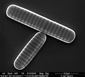
Figure 1: (Left to right, top to bottom) Thalassiosira pseudonana, Phaeodactylum tricornutum, Fragilariopsis cornutum, arctic food chain
Goal
Our goal is to optimize a way to predict which diatom species populations will increase and decrease as the ocean acidifies. Previous studies done by Dr. Jacob Valenzuela have identified a specific gene called the Na+(K+)/H+ antiporter that is upregulated in high carbon conditions in the diatom, Thalassiosira pseudonana (Thaps). Additional studies by Dr. Valenzuela have shown that Thaps are more resilient in high carbon conditions. Therefore, the presence of this gene in species of diatoms could be a good biomarker for identifying which diatoms will be resilient in the future. In brief, if a diatom has this gene, its population can handle more stress in higher carbon conditions.
To test whether the antiporter can be used as a biomarker, we must test to see if other species have this gene, and if so, how much is that gene being expressed in high vs. low carbon conditions. This could be done through RNA sequencing, which is expensive. However, it could be measured in a less costly way by optimizing a protocol to measure the expression of the antiporter through quantitative polymerase chain reaction (RT-qPCR). This process makes copies of a selected gene and measures how fast the number of copies is increasing. Since the process is exponential (the number of transcript copies should double every time) – the faster the number of genes increases, the higher the starting expression.
We aimed to optimize an RT-qPCR protocol to measure the expressions of the Na+(K+)/H+ antiporter in Thaps and other diatoms.
Process
The first step was to grow Thaps so we could extract the DNA and RNA. RNA expression reflects the environmental conditions of the organism, so we grew Thaps in high and low carbon conditions.
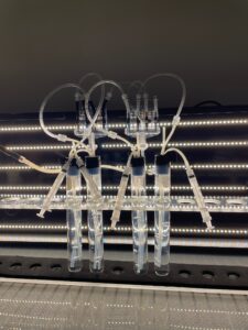
In parallel, we began designing primers, which are short single-stranded DNA that specifies which gene to amplify during PCR. We used a database created by the National Institute of Health, called Primer-BLAST, to find primers that had the potential to work. We also wanted to find orthologs (the same gene in another species) to see if the Na+(K+)/H+ antiporter also helps other diatoms be more resilient in high carbon conditions. We did this using the database created by EnsemblProtists and found many other diatoms with the antiporter. We decided to test Phaeodactylum tricornutum (Phaeo) and Fragilariopsis cylindrus (Frag) since we already had cultures of those diatoms and set them up to grow in high and low carbon conditions in mini-bioreactors.
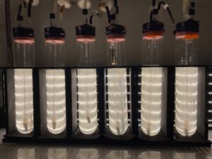
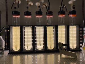
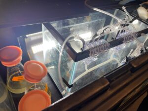
Figure 2: (Left to right) Large Thaps bioreactors day 1, large Thaps bioreactors day 4, Phaeo and Frag high carbon mini-reactors
Phaeo grew very well and multiplied very quickly, however, we were not able to grow Frag successfully in high and low carbon conditions because it is an arctic diatom and we did not have the proper facilities to grow it at 4°C while controlling the carbon flow. We decided to continue with the experiment using DNA and RNA from the stock cultures we already had that were grown only in ambient carbon conditions in addition to the Thaps DNA and RNA..
Figure 3: Frag cold room mini-reactors
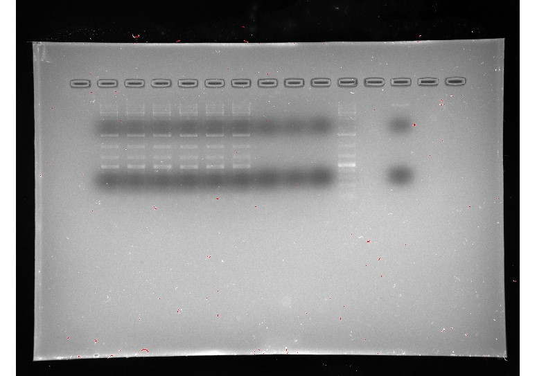
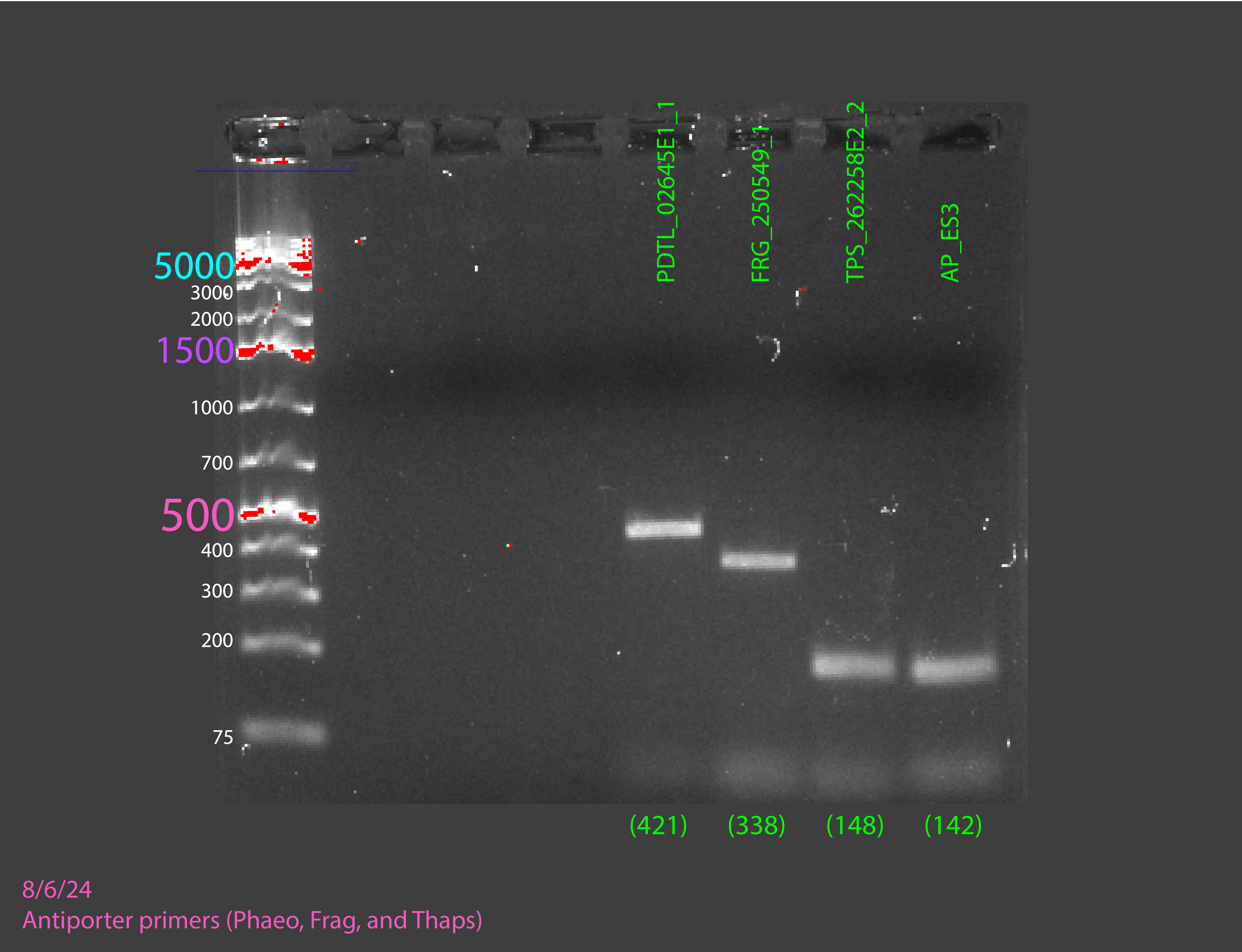
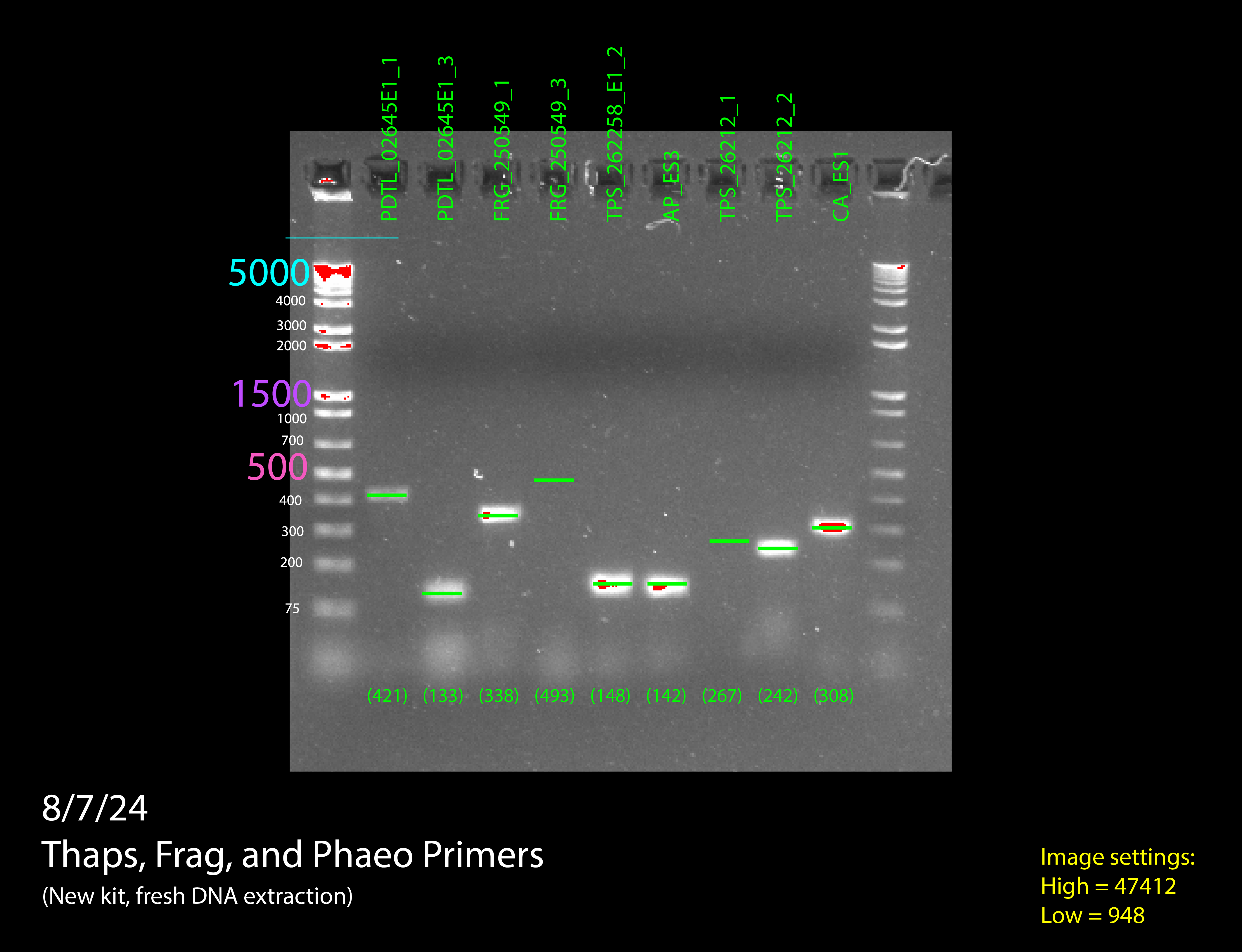
Once we had all the cultures we wanted to test primers done, we extracted DNA from them. With that DNA, we did a PCR (not RT-qPCR) to see if our primers had any possibility of working on the RNA without actually having to use RNA. This PCR would only tell us if the primers worked or not. We interpreted the results of the PCR by running a gel electrophoresis. If the bands of PCR product that showed up on the gel electrophoresis were sufficiently bright and in the right location, we would know that our primers worked, and we could move on to testing them on RNA.
Results
Our gels failed many times for many different reasons, but not because our primers weren’t working, but because of issues with the experiment itself. We had to adapt to the failures, adding more DNA, adding more primers, trying new ladders, redoing our DNA extractions, using fresh reagents, and editing our protocol, and on our sixth gel we got good bands and confirmed our primers worked, allowing us to move on to RT-PCR.
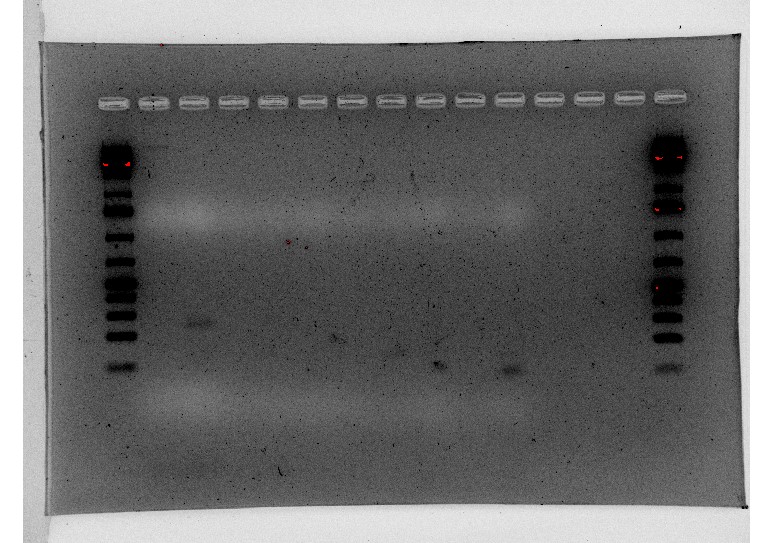
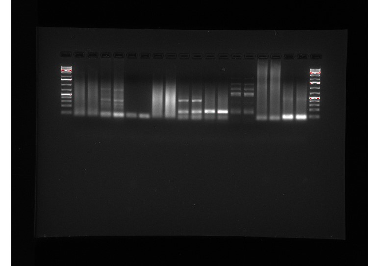
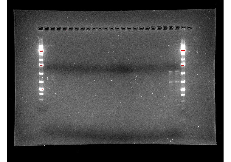
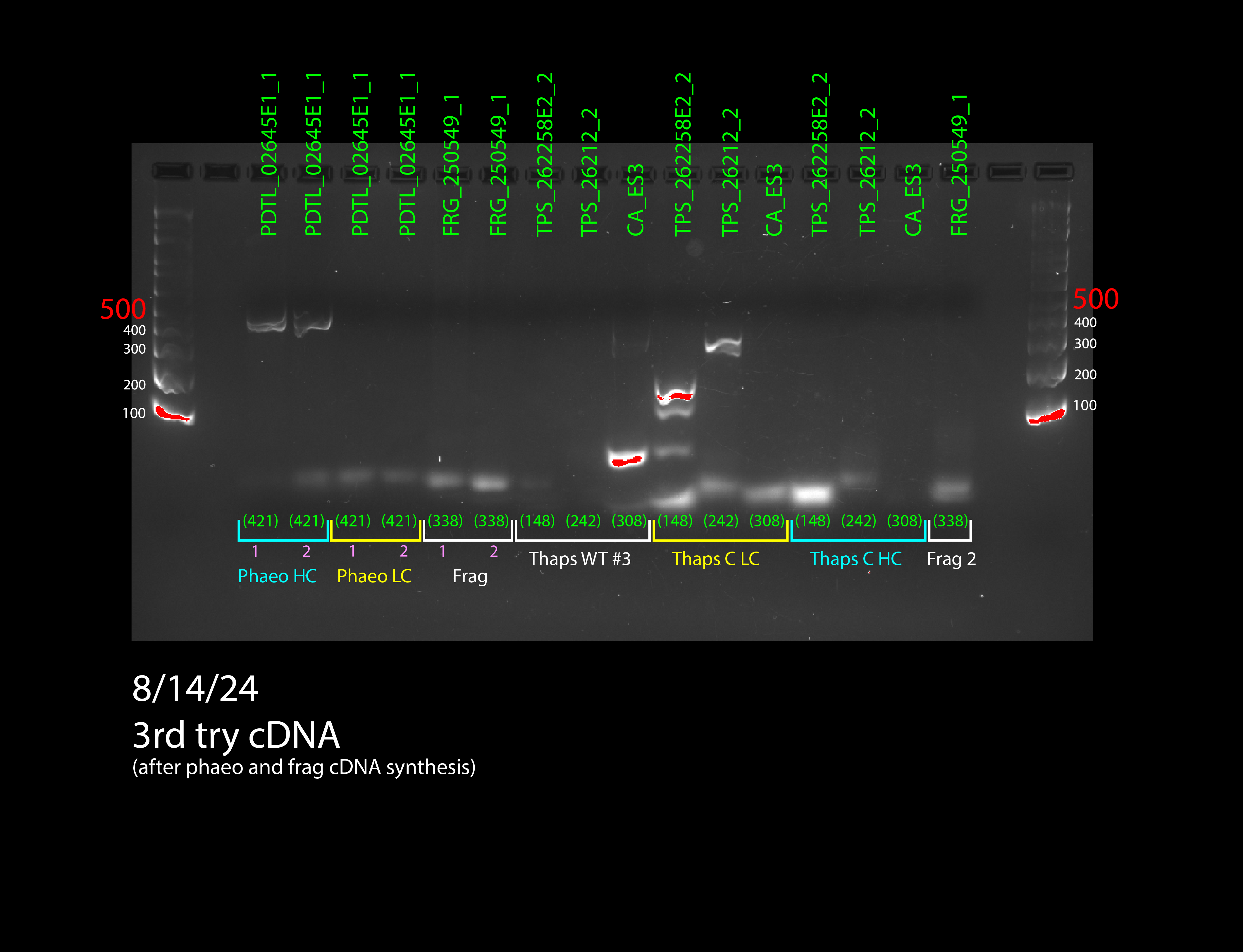
Figure 4: all DNA gel electrophoresis results
(In order) 7/23/24 PCR #1 (light), 7/23/24 PCR #2 (dark), 7/26/24 PCR #1 (dark), 7/26/24 PCR #2 (dark), 8/2/24 PCR #1 (dark), 8/2/24 PCR #2 (dark), 8/6/24 PCR #1 (dark) (annotated), 8/7/24 PCR #1 (dark) (annotated)
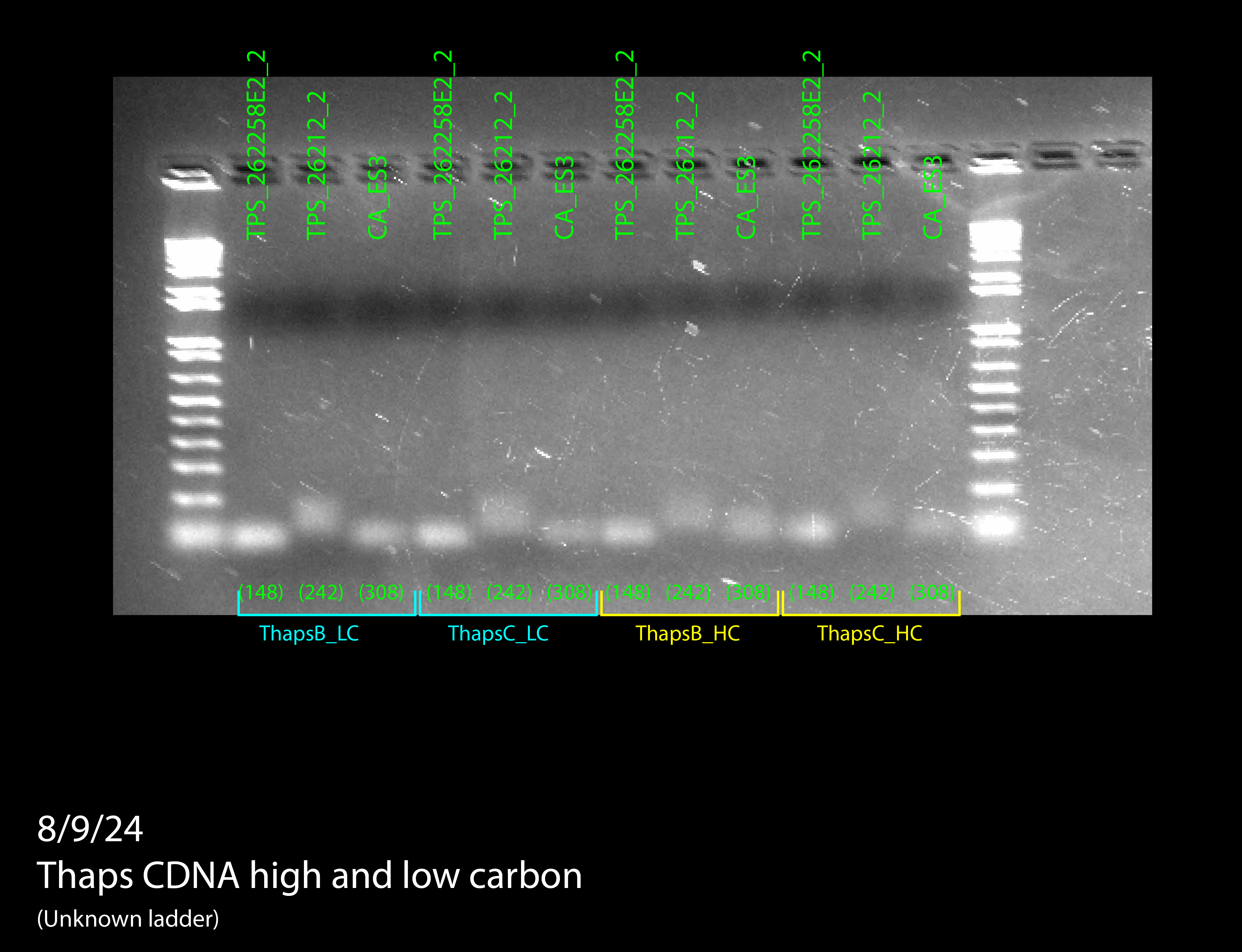
Then we moved onto the final step of the process: RT-qPCR. Since we had confirmation that our primers worked on cDNA, the primers were effective to measure expression in a quantitative way. The process for RT-qPCR is almost identical to normal PCR, except that a fluorescent dye is added to the PCR mix. This dye will bind to the copies of the gene that PCR creates and the ThermoCycler that the PCR happens in will measure the fluorescence over time, which is a proxy for how many copies of the gene there are. We need to look at how fast copies are made to see how much a gene is expressed. If a gene is highly expressed, the graph will increase quickly, while if a gene is not highly expressed, it will take some time for the graph to start increasing.
Figure 6: first RT-qPCR results
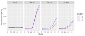
According to our graphs, we know our primers worked, but we’re unsure if our data is quantitative. We did our RT-qPCR on three different genes: the antiporter, a carbonic anhydrase gene, and an internal reference gene. The antiporter should have high expression in high carbon conditions and low expression in low carbon conditions. The carbonic anhydrase is supposed to have the opposite expression as the antiporter – it should be expressed highly in low carbon and lowly in high carbon. The internal reference gene is supposed to have the same expression regardless of the carbon conditions. We saw that low carbon was expressed more than high carbon regardless of which gene was being tested, which leads us to suspect that we unintentionally added more low carbon cDNA than high carbon cDNA. However, if we did add more low carbon cDNA, then all fluorescence for the low carbon PCR products should increase before it does for high carbon, but they both start increasing at the same time. This led us to very inconclusive results about what went wrong, so we decided to do it again.
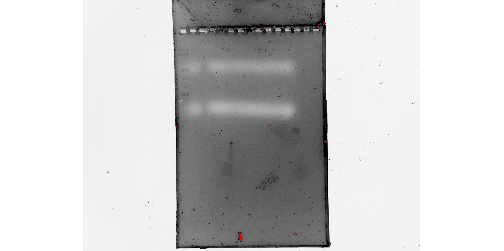
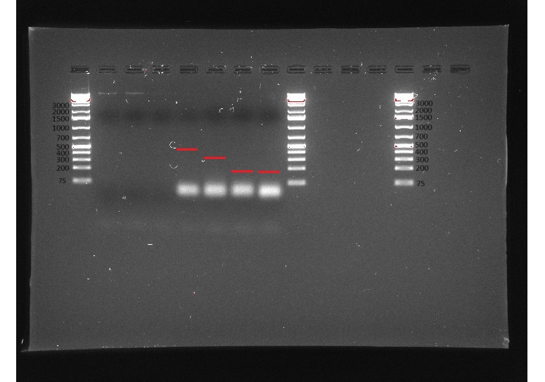
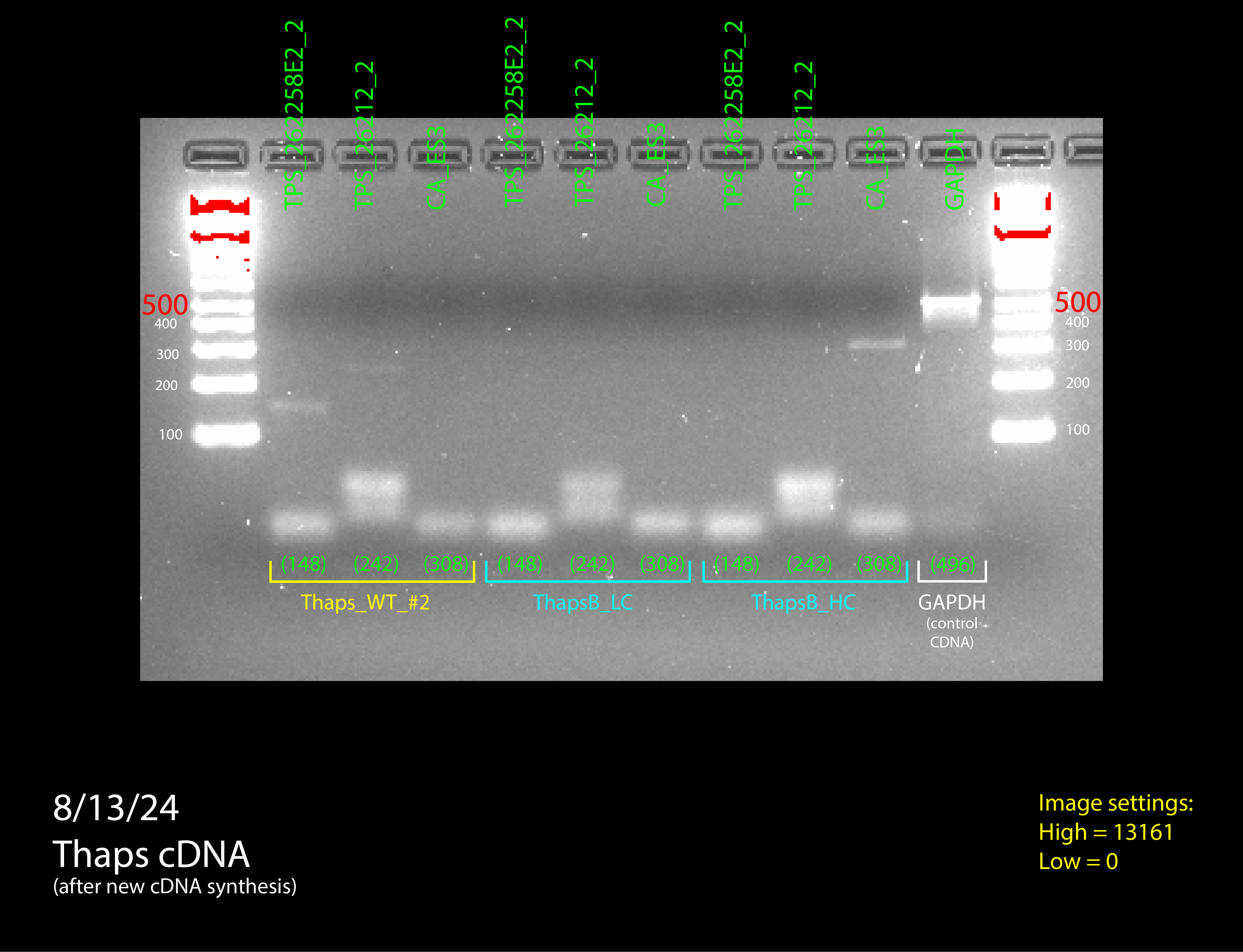
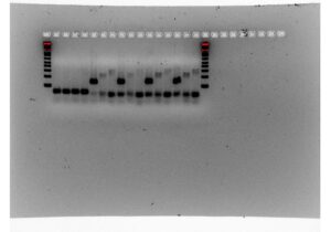
We tried doing a RT-qPCR three more times, however, each time we did it, we only got flat lines, meaning that the ThermoCycler wasn’t recording any fluorescence. Since we knew that there should be at least some fluorescence due to the previous RT-qPCR and other studies, there had to be something wrong with how we were doing the experiment itself. After trying the RT-qPCR with new RNA and new cDNA, we decided to do a gel electrophoresis on one of the failed PCR products to see if lack of amplification or lack of measurement was the issue. The gel electrophoresis was our most successful one yet, and since other people had successfully done RT-qPCRs on the ThermoCycler while we were troubleshooting, we knew the machine was working properly. Because of this, we were able to determine that the fluorescent dye in our SyberGreen Master Mix wasn’t working.
Figure 7: RT-qPCR product gel results
Although we weren’t able to measure the gene expression quantitatively, we were able to make working primers for internal reference and antiporter genes for Thaps. The next steps would be to redo the RT-qPCR with a working kit and higher quality RNA to reduce the chance for error. If the RT-qPCR graphs come out as expected, we can then move on to writing the official protocol for measuring the expression of the Na+(K+)/H+ antiporter in Thalassiosira pseudonana. Afterward we would focus on developing the same protocol and antiporter measurement techniques for other organisms, starting with Phaeodactylum tricornutum and Fragilariopsis cylindrus. If the antiporter is found to increase resilience in other species of diatoms, it could be used as a biomarker for increased resilience in high carbon conditions.
While we weren’t able to run a successful RT-qPCR by the end of the internship, the development of working internal reference primers for Thaps and experimenting with growing and making primers for Phaeo and Frag was a success!
Acknowledgements
Thank you so much to our mentors, Dr. Jacob Valenzuela and Dr. Chris Deutsch, for their guidance, encouragement, and support! Jake — we will miss your funny stories. Chris — we will miss your amazing baked goods. We had so much fun this summer and we learned a lot!
Thank you to Claudia Ludwig and Sarah Clemente for running the SEE programs and helping us develop our leadership and professional skills.
Thank you to everybody at ISB for being so kind and welcoming — we could not have done it without you!
References
Armbrust, E. V. (2009). The life of diatoms in the world’s oceans. Nature, 459(7244), 185–192. https://doi.org/10.1038/nature08057
Barker , S., & Ridgwell, A. (2012). Ocean Acidification . Nature news. https://www.nature.com/scitable/knowledge/library/ocean-acidification-25822734/
Liou, J. (2022, June 8). What is ocean acidification?. IAEA. https://www.iaea.org/newscenter/news/what-is-ocean-acidification
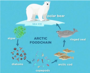
Observe the following food chain.Ice algae → Zooplankton →Arctic cod fish→ Seals→ Polar bearWhat will happen if ice melts and the ice algae population drops down? (n.d.). Byjus.com. https://byjus.com/question-answer/observe-the-following-food-chain-ice-algae-rightarrow-zooplankton-rightarrow-arctic-cod-fish-rightarrow-seals-1/
Valenzuela, J. J., Ashworth, J., Cusick, A., Abbriano, R. M., Armbrust, E. V., Hildebrand, M., Orellana, M. V., & Baliga, N. S. (2021). Diel transcriptional oscillations of a plastid antiporter reflect increased resilience of Thalassiosira pseudonana in elevated CO2. Frontiers in Marine Science, 8. https://doi.org/10.3389/fmars.2021.633225
Valenzuela, J. J., López García de Lomana, A., Lee, A., Armbrust, E. V., Orellana, M. V., & Baliga, N. S. (2018). Ocean acidification conditions increase resilience of marine diatoms. Nature Communications, 9(1). https://doi.org/10.1038/s41467-018-04742-3